Bayesian Spatial Modeling of School Disparities in Brunei Darussalam
Alvin Bong Jia Lok
VSRP, BAYESCOMP @ CEMSE-KAUST
https://alvinbjl.github.io/school-disparity-areal-model/presentation/
October 13, 2025
Introduction
Education is a foundational pillar of national development and its people. Key factors for quality education:
- Availability of school infrastructure
- Equitable access to schools
- Adequate teacher-to-student ratios
- Safe and inclusive learning environments
Introduction
Education is a foundational pillar of national development and its people. Key factors for quality education:
- Availability of school infrastructure
- Equitable access to schools
- Adequate teacher-to-student ratios
- Safe and inclusive learning environments
Several studies examined general aspects of education in Brunei [Ebil and Shahrill (2023); Abdul Latif, Matzin, and Escoto-Kemp (2021); Salbrina, Deterding, and Nur Raihan (2024); Mohamad et al. (2018).
First to examine through spatial methods & statistical models!
Study Focus
Main goal
Identify adminstrative regions in Brunei where school availability falls significantly below the national baseline.
This supports future policy planning and school placements.
Study Region: Brunei Darussalam
School Specification: Primary & Secondary Government (PUBLIC) schools
Region: 39 Mukim (sub-division of district)
Data
- Key data:
- School counts (2018; latest detailed data)
- population & youth population (2021; census evey 10 years)
- administrative boundaries
- Median house prices (1993–2025), used as socioeconomic covariate
- Data sourced from
BruneiverseGitHub page mainly viabruneimapR package (Jamil 2025; Jamil et al. 2025) - Missing house prices imputed via INLA-based Gaussian model; preferred over manual imputation
- House prices are partially simulated estimates, may not fully reflect market values
- Raw school data in points; grouped into areal (mukim)
Methods
Bayesian Spatial Model
Let \(Y_i\) and \(E_i\) denote the observed and expected counts of schools, respectively, in mukim \(i \in \{1, \dotsc, n\}\). Let \(\theta_i\) represent the relative abundance (RA) of schools in mukim \(i\), analogous to a relative risk in disease mapping.
Bayesian hierarchical model + BYM
\[ Y_i \mid \theta_i \sim \text{Poisson}(E_i \cdot \theta_i), \quad i = 1, \dotsc, n \]
\[ \log(\theta_i) = \beta_0 + \beta_1 \cdot \text{pop youth}_i + \beta_2 \cdot \text{area}_i + \beta_3 \cdot \text{hp}_i + u_i + v_i, \]
Methods
Bayesian Spatial Model
Bayesian hierarchical model + BYM
\[ Y_i \mid \theta_i \sim \text{Poisson}(E_i \cdot \theta_i), \quad i = 1, \dotsc, n \]
\[ \log(\theta_i) = \beta_0 + \beta_1 \cdot \text{pop youth}_i + \beta_2 \cdot \text{area}_i + \beta_3 \cdot \text{hp}_i + u_i + v_i, \]
- \(\beta_0\) is the intercept,
- \(\beta_1\), \(\beta_2\), and \(\beta_3\) are regression coefficients for the standardized covariates:
- \(\text{pop youth}_i\): population of youth aged 0-24 (in units of 10,000),
- \(\text{area}_i\): mukim size (in units of 10 km²),
- \(\text{hp}_i\): median house price (in BND $1,000,000),
- \(u_i\) is a structured spatial effect, (CAR) prior \(u_i \mid u_{-i} \sim \mathcal{N}(\bar{u}_{\delta_i}, \frac{1}{\tau_u n_{\delta_i}})\)
- \(v_i\) is an unstructured random effect, \(v_i \sim \text{Normal}(0, \frac{1}{\tau_v})\)
Methods
Neighbour
Spatial random effect \(u_i\) uses Queen Contiguity neighborhood (adjacency)
Estimation
Model fitting performed using INLA (Rue, Martino, and Chopin 2009).
Spatial autocorrelation
Model adequacy (spatial structure) is assessed by spatial autocorrelation (Global Moran’s I) of residual: \[residual_i = \dfrac{Y_i - \mu_i}{\sqrt{\mu_i}} = \dfrac{Y_i - E_i \cdot \theta_i}{\sqrt{E_i \cdot \theta_i}},\]
Methods
Spatial autocorrelation (cont.)
For each mukim in the study area \(i, j = 1, 2, \ldots, N\). The Moran’s I test statistic is defined as follows:
\[ I = \frac{N}{\sum_{i=1}^N \sum_{j=1}^N w_{ij}} \frac{\sum_{i=1}^N \sum_{j=1}^N w_{ij} (x_i - \bar{x})(x_j - \bar{x})}{\sum_{i=1}^N (x_i - \bar{x})^2} \in [-1,1], \]
- \(x_i\) is the Pearson residual in mukim \(i\),
- \(\bar{x}\) is the mean residual per mukim,
- \(w_{ij}\) is the spatial weight between mukims \(i\) and \(j\).
Methods
Spatial autocorrelation (cont.)
Same Queen Contiguity neighbour is used.
Central Limit Theorem (CLT) employed for hypthesis test for significance of the Moran’s I statistic (z-scores):
- \(H_0: I = 0\) (no spatial autocorrelation),
- \(H_1: I \neq 0\) (presence of spatial autocorrelation).
Results
Exploratory Data Analysis
- Mukims with higher schools count are concentrated in the coastal region near South China Sea
- As expected, schools are more clustered in Brunei-Muara District (northeast of the mainland), Brunei’s most populated and urbanized district
Model
Model
| Term | Mean | 2.5% | 97.5% | Significant |
|---|---|---|---|---|
| (Intercept) | 0.824 | 0.430 | 1.215 | Yes |
| pop_y | -0.123 | -0.163 | -0.083 | Yes |
| area | 0.018 | 0.001 | 0.036 | Yes |
| hp | 0.001 | -0.002 | 0.003 | No |
- School availability in rural mukims seem to be adequate
- Significant negative relationship between population youth and school counts
- Higher RA values in inland (rural) mukims than coastal areas with larger population
- Positive relationship between schools counts and mukim size
- House price NOT significant
- No clear “socio-economic” disparity (house price as proxy)
Non-exceedence Probability
- Disparitiy in Mukim Sengkurong, Gadong A & B, Berakas B, and Mentiri
- Fewer schools than expected relative to population size
- Mukim Sengkurong & Mentiri encompass new government housing developments (Perpindahan Lugu, Perpindahan Tanah Jambu)
- Potential planning gap in schools infrastructure
Spatial Autocorrelation
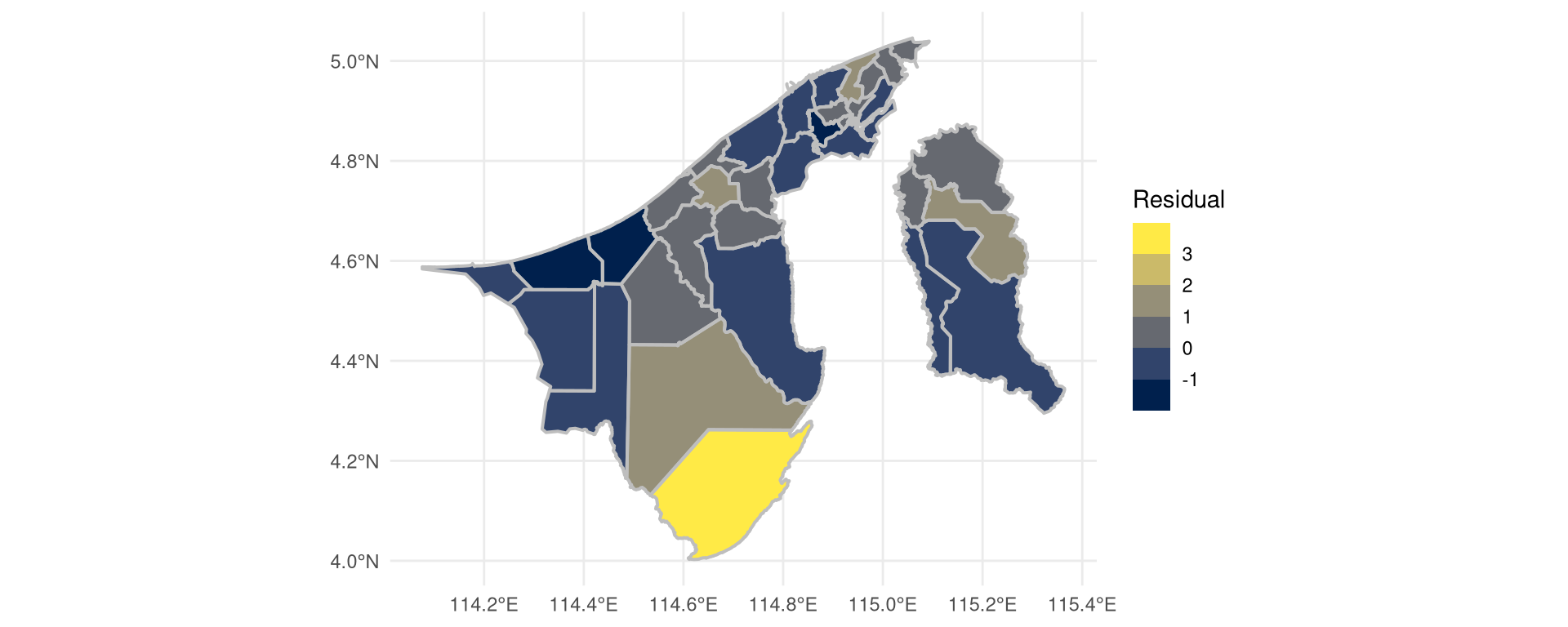
- Global Moran’s I: \(0.213\) (p=0.0123 < 0.05)
- Statistically significant evidence to reject the null hypothesis of no spatial autocorrelation in the residuals
- Some spatial dependencies but not “too high”
- Model is “moderately” good
Conclusion
- Negative relationship between population size and relative school
- Enough infrastructure in rural areas
- Potetntial gaps in Mukim Sengkurong, Gadong A & B, Berakas B, and Mentiri
Limitations
- Old school data (2018)
- Population not age-standardized
- Housing price is listing price & partially simulated
- Only focus on public schools
- Only consider “count” of schools, (school sizes, travel distance not accounted)
References
Abdul Latif, Siti Norhedayah, Rohani Matzin, and Aurelia Escoto-Kemp. 2021. “The Development and Growth of Inclusive Education in Brunei Darussalam.” Globalisation, Education, and Reform in Brunei Darussalam, 151–75. https://doi.org/10.1007/978-3-030-77119-5_8.
Ebil, Syazana, and Masitah Shahrill. 2023. “Overview of Education in Brunei Darussalam.” In International Handbook on Education in South East Asia, 1–21. Springer. https://doi.org/10.1007/978-981-16-8136-3_46-1.
Jamil, Haziq. 2025. Bruneimap: Maps and Spatial Data of Brunei (R Package Version 0.3.1.9001). https://bruneiverse.github.io/bruneimap/.
Jamil, Haziq, Amira Barizah Noorosmawie, Hafeezul Waezz Rabu, and Lutfi Abdul Razak. 2025. “From Archives to AI: Residential Property Data Across Three Decades in Brunei Darussalam.” Data in Brief, March. https://doi.org/10.1016/j.dib.2025.111505.
Mohamad, Hanapi, Rosyati M Yaakub, Emma Claire Pearson, and Jennifer Tan Poh Sim. 2018. “Towards Wawasan Brunei 2035: Early Childhood Education and Development in Brunei Darussalam.” International Handbook of Early Childhood Education, 551–67. https://doi.org/10.1007/978-94-024-0927-7_25.
Rue, Håvard, Sara Martino, and Nicolas Chopin. 2009. “Approximate Bayesian Inference for Latent Gaussian Models by Using Integrated Nested Laplace Approximations.” Journal of the Royal Statistical Society Series B: Statistical Methodology 71 (2): 319–92.
Salbrina, Sharbawi, David Deterding, and Mohamad Nur Raihan. 2024. “Education in Brunei.” In Brunei English: A New Variety in a Multilingual Society, 17–32. Springer. https://doi.org/10.1007/978-3-031-60303-7_2.
![]()